Examine notebook used to visualize results

First we will load the endpoint name, training time, prediction length and seom of the data

%store -r
print('endpoint name ', endpoint_name)
print('end training', end_training)
print('prediction_length', prediction_length)

endpoint name  DeepAR-forecast-taxidata-2019-11-30-16-26-45-053
end training 2019-05-06 00:00:00
prediction_length 14

Sample data being used:

print('data sample')
ABB.head(5)

data sample

	green	yellow	full_fhv
ts_resampled
2018-01-01	23292	237118	702058.0
2018-01-02	23222	238152	547447.0
2018-01-03	26417	266992	583735.0
2018-01-04	6519	122222	354626.0
2018-01-05	27453	265212	699966.0

This next cell creates the predictor using the endpoint_name. Ideally we’d have the DeepARPredictor in a seperate .py rather than repeated in the two notebooks.

import sagemaker
from sagemaker import get_execution_role
from sagemaker.tuner import HyperparameterTuner
import numpy as np
import json
import pandas as pd

import warnings
warnings.simplefilter(action='ignore', category=FutureWarning)

class DeepARPredictor(sagemaker.predictor.RealTimePredictor):

    def __init__(self, *args, **kwargs):
        super().__init__(*args, content_type=sagemaker.content_types.CONTENT_TYPE_JSON, **kwargs)

    def predict(self, ts, cat=None, dynamic_feat=None,
                num_samples=100, return_samples=False, quantiles=["0.1", "0.5", "0.9"]):
        """Requests the prediction of for the time series listed in `ts`, each with the (optional)
        corresponding category listed in `cat`.

        ts -- `pandas.Series` object, the time series to predict
        cat -- integer, the group associated to the time series (default: None)
        num_samples -- integer, number of samples to compute at prediction time (default: 100)
        return_samples -- boolean indicating whether to include samples in the response (default: False)
        quantiles -- list of strings specifying the quantiles to compute (default: ["0.1", "0.5", "0.9"])

        Return value: list of `pandas.DataFrame` objects, each containing the predictions
        """
        prediction_time = ts.index[-1] + 1
        quantiles = [str(q) for q in quantiles]
        req = self.__encode_request(ts, cat, dynamic_feat, num_samples, return_samples, quantiles)
        res = super(DeepARPredictor, self).predict(req)
        return self.__decode_response(res, ts.index.freq, prediction_time, return_samples)

    def __encode_request(self, ts, cat, dynamic_feat, num_samples, return_samples, quantiles):
        instance = series_to_dict(ts, cat if cat is not None else None, dynamic_feat if dynamic_feat else None)

        configuration = {
            "num_samples": num_samples,
            "output_types": ["quantiles", "samples"] if return_samples else ["quantiles"],
            "quantiles": quantiles
        }

        http_request_data = {
            "instances": [instance],
            "configuration": configuration
        }

        return json.dumps(http_request_data).encode('utf-8')

    def __decode_response(self, response, freq, prediction_time, return_samples):
        # we only sent one time series so we only receive one in return
        # however, if possible one will pass multiple time series as predictions will then be faster
        predictions = json.loads(response.decode('utf-8'))['predictions'][0]
        prediction_length = len(next(iter(predictions['quantiles'].values())))
        prediction_index = pd.DatetimeIndex(start=prediction_time, freq=freq, periods=prediction_length)
        if return_samples:
            dict_of_samples = {'sample_' + str(i): s for i, s in enumerate(predictions['samples'])}
        else:
            dict_of_samples = {}
        return pd.DataFrame(data={**predictions['quantiles'], **dict_of_samples}, index=prediction_index)

    def set_frequency(self, freq):
        self.freq = freq

def encode_target(ts):
    return [x if np.isfinite(x) else "NaN" for x in ts]

def series_to_dict(ts, cat=None, dynamic_feat=None):
    """Given a pandas.Series object, returns a dictionary encoding the time series.

    ts -- a pands.Series object with the target time series
    cat -- an integer indicating the time series category

    Return value: a dictionary
    """
    obj = {"start": str(ts.index[0]), "target": encode_target(ts)}
    if cat is not None:
        obj["cat"] = cat
    if dynamic_feat is not None:
        obj["dynamic_feat"] = dynamic_feat
    return obj

predictor = DeepARPredictor(endpoint_name)

import matplotlib
import matplotlib.pyplot as plt

def plot(
    predictor,
    target_ts,
    cat=None,
    dynamic_feat=None,
    forecast_date=end_training,
    show_samples=False,
    plot_history=7 * 12,
    confidence=80,
    num_samples=100,
    draw_color='blue'
):
    print("Calling endpoint to generate {} predictions starting from {} ...".format(target_ts.name, str(forecast_date)))
    assert(confidence > 50 and confidence < 100)
    low_quantile = 0.5 - confidence * 0.005
    up_quantile = confidence * 0.005 + 0.5

    # we first construct the argument to call our model
    args = {
        "ts": target_ts[:forecast_date],
        "return_samples": show_samples,
        "quantiles": [low_quantile, 0.5, up_quantile],
        "num_samples": num_samples
    }


    if dynamic_feat is not None:
        args["dynamic_feat"] = dynamic_feat
        fig = plt.figure(figsize=(20, 6))
        ax = plt.subplot(2, 1, 1)
    else:
        fig = plt.figure(figsize=(20, 3))
        ax = plt.subplot(1,1,1)

    if cat is not None:
        args["cat"] = cat
        ax.text(0.9, 0.9, 'cat = {}'.format(cat), transform=ax.transAxes)

    # call the end point to get the prediction
    prediction = predictor.predict(**args)

    # plot the samples
    mccolor = draw_color
    if show_samples:
        for key in prediction.keys():
            if "sample" in key:
                prediction[key].asfreq('D').plot(color='lightskyblue', alpha=0.2, label='_nolegend_')

    # the date didn't have a frequency in it, so setting it here.
    new_date = pd.Timestamp(forecast_date, freq='d')
    target_section = target_ts[new_date-plot_history:new_date+prediction_length]
    target_section.asfreq('D').plot(color="black", label='target')
    plt.title(target_ts.name.upper(), color='darkred')

    # plot the confidence interval and the median predicted
    ax.fill_between(
        prediction[str(low_quantile)].index,
        prediction[str(low_quantile)].values,
        prediction[str(up_quantile)].values,
        color=mccolor, alpha=0.3, label='{}% confidence interval'.format(confidence)
    )
    prediction["0.5"].plot(color=mccolor, label='P50')
    ax.legend(loc=2)

    # fix the scale as the samples may change it
    ax.set_ylim(target_section.min() * 0.5, target_section.max() * 1.5)

    if dynamic_feat is not None:
        for i, f in enumerate(dynamic_feat, start=1):
            ax = plt.subplot(len(dynamic_feat) * 2, 1, len(dynamic_feat) + i, sharex=ax)
            feat_ts = pd.Series(
                index=pd.DatetimeIndex(start=target_ts.index[0], freq=target_ts.index.freq, periods=len(f)),
                data=f
            )
            feat_ts[forecast_date-plot_history:forecast_date+prediction_length].plot(ax=ax, color='g')

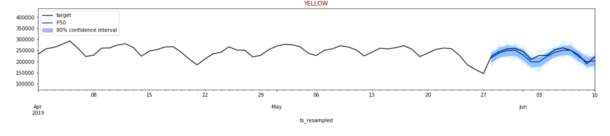
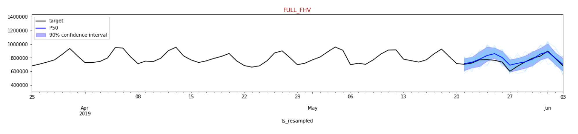
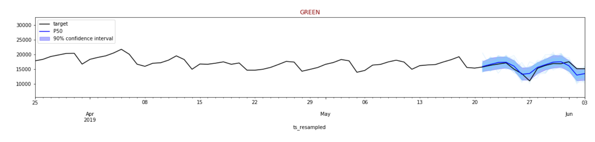
Let’s interact w/ the samples and forecast values now.

from __future__ import print_function
from ipywidgets import interact, interactive, fixed, interact_manual
import ipywidgets as widgets
from ipywidgets import IntSlider, FloatSlider, Checkbox, RadioButtons
import datetime

style = {'description_width': 'initial'}

@interact_manual(
    series_type=RadioButtons(options=['full_fhv', 'yellow', 'green'], value='yellow', description='Type'),
    forecast_day=IntSlider(min=0, max=100, value=21, style=style),
    confidence=IntSlider(min=60, max=95, value=80, step=5, style=style),
    history_weeks_plot=IntSlider(min=1, max=20, value=4, style=style),
    num_samples=IntSlider(min=100, max=1000, value=100, step=500, style=style),
    show_samples=Checkbox(value=True),
    continuous_update=False
)

def plot_interact(series_type, forecast_day, confidence, history_weeks_plot, show_samples, num_samples):
    plot(
        predictor,
        target_ts=ABB[series_type].asfreq(freq='d', fill_value=0),
        forecast_date=end_training + datetime.timedelta(days=forecast_day),
        show_samples=show_samples,
        plot_history=history_weeks_plot * prediction_length,
        confidence=confidence,
        num_samples=num_samples
    )

interactive(children=(RadioButtons(description='Type', index=1, options=('full_fhv', 'yellow', 'green'), value…

Testing and Understanding the results

You can test the results and see different results. Here are some examples below: